Understanding scaling factor in attention computation
Deriving the scaling factor 1/sqrt(d_k) and using simulation to observe its effect
Attention Formula
Below is the Attention formula in the “Attention is all you need” paper. We will attempt to derive and understand the purpose of the scaling factor in the denominator. Later we will simulate what happens to attention values if we do not include the scaling term.
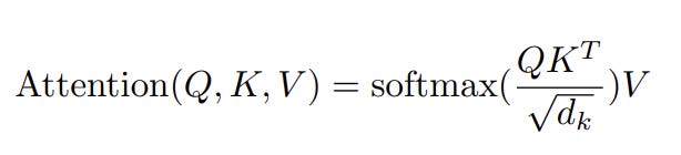
With respect to formula, the author reasons that dot products grow large in magnitude making the softmax peak highly as seen below.
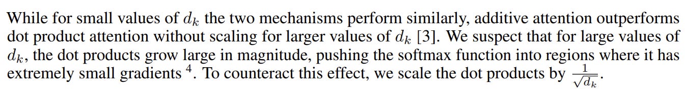
As for why the use of this particular value for scaling the author illustrates with below observation.

Derivation:
Lets do a complete derivation using the authors assumption. To complete the derivation we will need the below properties of expectation and variance of random variables.
Below equations assume that X and Y are independent random variables.
Let’s derive a new property from the above properties. We will start with substituting XY in place of X in property 3.
If X and Y are independent then X^2 and Y^2 will also be independent so using property 2 in the above eqn we get
Again using property 2 above
Dot Product between Q and K
Matrix multiplication between Q and K.T( we will use K.T to mean transpose of K) which we will write as Q@K.T (we will use A@B to mean matrix multiplication) represents dot product between every row of Q with every row of K.
Expanding, let’s assume we are doing attention computation on a sequence of 100 tokens. Q is a matrix of shape (100, 64) having 100 rows and 64 columns. Row i represent the query vector of i_th input token. Similarly K is a matrix of shape (100, 64) where there are 100 rows and 64 columns with each row representing the key vector representation of each of the token.
The purpose of attention layer is computing how well should each token attend to every other token in the input sequence of 100 tokens. How much should token 1 attend to token 2 . As with everything it will be scalar real value and this value is computed by dot product between the 1st row of Q and 2nd row of K. If we want to know how much token 5 should attend to token 11, we will do dot product between row 5 of Q and row 11 of K. Each of the two selected rows are vectors of size 64 and dot product between them will give a single scalar value. 64 is the size of each of the heads in the multi headed attention introduced in the paper. After the attention, 8 of these outputs from 8 of the heads of size 64 are concatenated to give 512 dim vector as final output of attention layer.
Calculating attention value between every token pair requires dot product between every row of Q with every row of K. This can be done by doing matrix multiplication between Q and K.T . One intuitive way to remember this is connect that A@B is dot product between rows and cols of A and B respectively, so when we want dot product between rows and rows we simply transpose the matrix B. This leads to A@B.T giving dot product between every row of A and B.
The result of the matrix multiplication Q@K.T will be a square matrix of shape (100,100). So the element (i,j) in this matrix represent the dot product between row i of Q and col j of K and it also means how much should token number i attend to token number j.
Elements of attention matrix
Lets zoom in on the value in the row i and col j of the Q@K.T matrix and understand its properties.
Let the mean and variance of q_in and k_jn be mean = 0 and var = 1.
Now in step 1 we will apply variance on both sides.
Applying property 5 from properties list, we can take the summation out,
Applying property 6 from properties list
Applying assumption 1 and 2 we can replace the expectations as 0.
Applying above property in step to step 4 to get
Using the values of var from assumption 1 and 2
We will now replace 64 with d_k since that is what d_k represents - the hidden dim of one of the heads in multi head attention.
Here comes the main trick, we can see that the variance is directly proportional to d_k. If we want to not scale the variance with d_k we can divide by d_k on both sides
Using property 4 we can take d_k inside Var on LHS
If we also keep both the variances of q and k close to 1 then the variance of attention scores will be close to 1 and this keeps the softmax computation stable without spiking values and training dynamics stable. Finally,
Simulation of attention values with and without the scaling constant
Full code in colab at link.
We will see how the attention values change with and without scaling. Below is the code used in computing softmax and also generating attention values given number of tokens in sequence and the dim d_k which is written as h_dim.
def calc_softmax(x: np.ndarray) -> np.ndarray:
    '''Compute softmax with numerical stability.'''
    if x.ndim != 2:
        raise ValueError(”expected 2D array”)
    x_centered = x - np.max(x, axis=1, keepdims=True)
    exp_x = np.exp(x_centered)
    return exp_x / np.sum(exp_x, axis=1, keepdims=True)

def run_experiment(n_tok: int, h_dim: int) -> tuple:
    '''
    Run single experiment: generate Q, K matrices and compute attention distributions.

    Args:
        n_tok: Number of tokens
        h_dim: Hidden dimension

    Returns:
        Tuple of (unscaled_attention, scaled_attention) softmax matrices
    '''
    # Generate random query and key matrices
    Q = rng.normal(0, 1, size=(n_tok, h_dim))
    K = rng.normal(0, 1, size=(n_tok, h_dim))

    # Compute attention scores (dot product)
    A = Q @ K.T # unscaled attention
    A_scaled = A / np.sqrt(h_dim) # scaled attention

    # Apply softmax
    A_softmax = calc_softmax(A)
    A_scaled_softmax = calc_softmax(A_scaled)

    return A_softmax, A_scaled_softmax
I will use n_tok = 50 and h_dim = 64 for the simulation and showcase the trend. We will use top_p_95 metric and heatmap to showcase the simulation results.
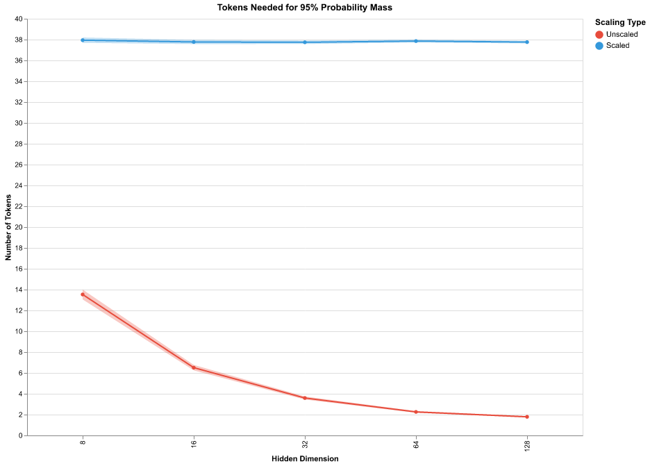
After applying softmax to the dot product values for each row we have sum of each row equal to 1. So we can treat them as probability density and by top_p_95 we calculate the minimum number of probability values from the row I need to accumulate a cumulative probability mass of 0.95 . So, we sort the row first in decreasing order and choose the first n elements whose sum crosses the threshold 0.95 - we call this number n as top_p_95. If the probability mass is concentrated in a few tokens then we get small values of top_p_95 and if it is well spread we will get larger values. In the below chart we see that on average for the scaled version we need top 38 token scores out of 50 to bring the cumulative sum of scores to 0.95 whereas for unscaled we see that it goes to 2 as the dim increases to 128 meaning the sum of attention scores of the top 2 tokens take up 0.95 .
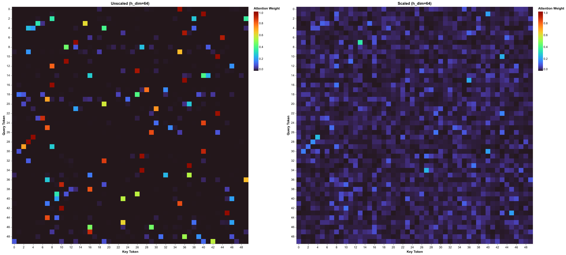
For the heatmap, since we have 50 tokens and the attention matrix will 50x50 matrix where each value will be between 0 to 1, the value is shown by the color shade. We will notice that in the unscaled heatmap for every row there is usually only one or two squares which have bright color and others are close to black. Whereas for the scaled heatmap we notice that there are not bright colors and there is good distribution of attention score in each row.